Introduction to forecasting with FB Prophet
Back to snippetsProphet is a forecasting tool developed by Facebook to quickly forecast time series data, available in R and Python. In this post I'll walk you through a quick example of how to forecast U.S. candy sales using Prophet and Python.
First, we'll read in the data, which shows the 'industrial production index', or INDPRO (detail here) for candy in the U.S. You can download the data in our github repository here.
#import libraries
import pandas as pd
import numpy as np
import matplotlib.pyplot as plt
from fbprophet import Prophet
#read in and preview our data
df = pd.read_csv('./datasets/candy_production.csv')
df.head()
| observation_date | IPG3113N | |
|---|---|---|
| 0 | 1972-01-01 | 85.6945 |
| 1 | 1972-02-01 | 71.8200 |
| 2 | 1972-03-01 | 66.0229 |
| 3 | 1972-04-01 | 64.5645 |
| 4 | 1972-05-01 | 65.0100 |
Great, so as we can see, we now have data showing U.S. candy production (normalized against 2012=100 in this dataset), which we can use as an input for our time series forecasting model with Prophet. Next, we'll need to do a little bit of cleaning to prep the data for Prophet.
#rename date column ds, value column y per Prohet specs
df.rename(columns={'observation_date': 'ds'}, inplace=True)
df.rename(columns={'IPG3113N': 'y'}, inplace=True)
#ensure our ds value is truly datetime
df['ds'] = pd.to_datetime(df['ds'])
#filtering here on >=1995, just to pull the last ~20 years of production information
start_date = '01-01-1995'
mask = (df['ds'] > start_date)
df = df.loc[mask]
Next, we can load our dataframe, df, into Prophet, and set a window for # of days we want it to predict
#initialize Prophet
m = Prophet()
#point towards dataframe
m.fit(df)
#set future prediction window of 2 years
future = m.make_future_dataframe(periods=730)
#preview our data -- note that Prophet is only showing future dates (not values), as we need to call the prediction method still
future.tail()
| ds | |
|---|---|
| 996 | 2019-07-28 |
| 997 | 2019-07-29 |
| 998 | 2019-07-30 |
| 999 | 2019-07-31 |
| 1000 | 2019-08-01 |
Next, we can call the predict method, which will assign each row in our 'future' dataframe a predicted value, which it names yhat. Additionally, it will show lower/upper bounds of uncertainty, called yhat_lower and yhat_upper.
forecast = m.predict(future)
forecast[['ds', 'yhat', 'yhat_lower', 'yhat_upper']].tail()
| ds | yhat | yhat_lower | yhat_upper | |
|---|---|---|---|---|
| 996 | 2019-07-28 | 117.796140 | 111.591576 | 123.519210 |
| 997 | 2019-07-29 | 117.016641 | 110.999394 | 122.908126 |
| 998 | 2019-07-30 | 116.001765 | 109.887603 | 122.016393 |
| 999 | 2019-07-31 | 114.757009 | 108.375085 | 121.465374 |
| 1000 | 2019-08-01 | 113.293294 | 107.234872 | 119.295134 |
We now have an initial time series forecast using Prophet, we can plot the results as shown below:
fig1 = m.plot(forecast)
fig1
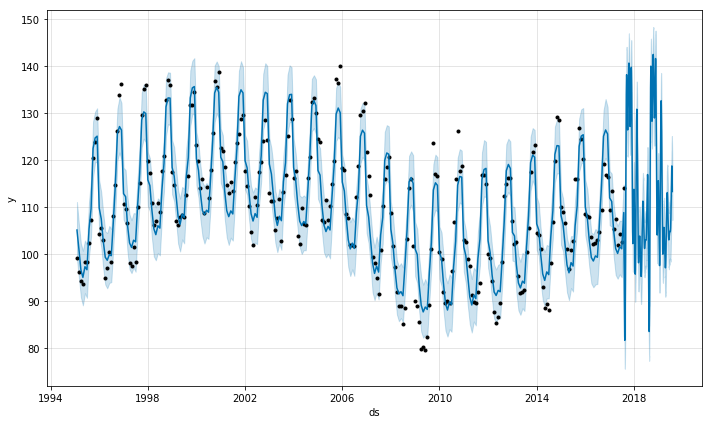
fig2 = m.plot_components(forecast)
fig2
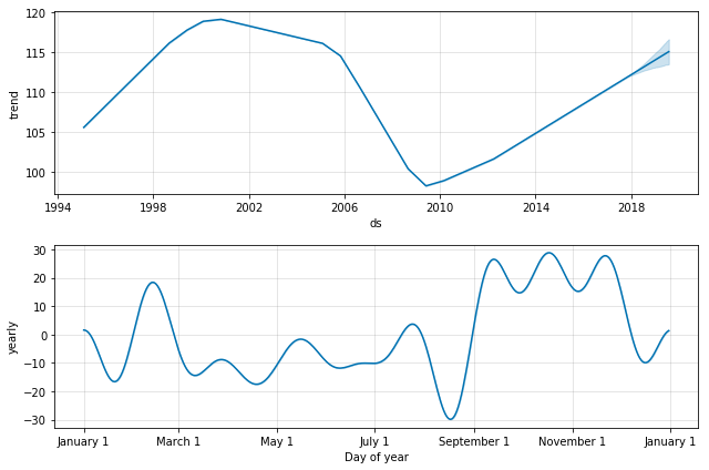
Here we can see at a high-level production is expected to continue it's upward trend over the next couple of years. Additionally, we can see the spikes in production for the various U.S. holidays (Valentine's Day, Halloween, Christmas). The Jupyter notebook used in this exercise can be found in our github repository here.
For more in depth reading, would recommend checking out the docs, as they're pretty easy to understand with additional detail/examples.