Calculating Value at Risk (VaR) of a Stock Portfolio using Python

February 2020

What is Value at Risk (VaR)?

Value at Risk (VaR) is a statistic used to try and quantify the level of financial risk within a firm or portfolio over a specified time frame. VaR provides an estimate of the maximum loss from a given position or portfolio over a period of time, and you can calculate it across various confidence levels.

Estimating the risk of a portfolio is important to long-term capital growth and risk management, particularly within larger firms or institutions. VaR is typically framed as something like this:

"We have a portfolio VaR of 250,000 USD over the next month at 95% confidence."
This means that, with 95% confidence, we can say that the portfolio's loss will not exceed 250,000 USD in a month.

In this post I'll walk you through the steps to calculate this metric across a portfolio of stocks.

How is VaR calculated?

There are two main ways to calculate VaR:

Using Monte Carlo simulation
Using the variance-covariance method

In this post, we'll focus on using the second method, variance-covariance. In short, the variance-covariance method looks at historical price movements (standard deviation, mean price) of a given equity or portfolio of equities over a specified lookback period. It then uses probability theory to calculate the maximum loss within your specified confidence interval. You can read more details here, but we'll calculate it step by step below using Python.

Before we get started, note that the standard VaR calculation assumes the following:

Normal distribution of returns - VaR assumes the returns of the portfolio are normally distributed. This is of course not realistic for most assets, but allows us to develop a baseline using a much more simplistic calculation.
(Modifications can be made to VaR to account for different distributions, but here we'll focus on the standard VaR calculation).
Standard market conditions - Like many financial instruments, VaR is best used for considering loss in standard markets, and is not well-suited for extreme/outlier events.

Steps to calculate the VaR of a portfolio

In order to calculate the VaR of a portfolio, you can follow the steps below:

Calculate periodic returns of the stocks in the portfolio
Create a covariance matrix based on the returns
Calculate the portfolio mean and standard deviation

(weighted based on investment levels of each stock in portfolio)

Calculate the inverse of the normal cumulative distribution (PPF) with a specified confidence interval, standard deviation, and mean
Estimate the value at risk (VaR) for the portfolio by subtracting the initial investment from the calculation in step (4)

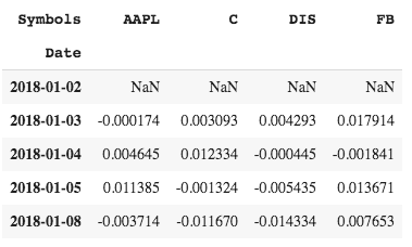
1) Calculate periodic returns of the stocks in the portfolio

import pandas as pd
from pandas_datareader import data as pdr
import fix_yahoo_finance as yf
import numpy as np
import datetime as dt

# Create our portfolio of equities
tickers = ['AAPL','FB', 'C', 'DIS']

# Set the investment weights (I arbitrarily picked for example)
weights = np.array([.25, .3, .15, .3])

# Set an initial investment level
initial_investment = 1000000

# Download closing prices
data = pdr.get_data_yahoo(tickers, start="2018-01-01", end=dt.date.today())['Close']

#From the closing prices, calculate periodic returns
returns = data.pct_change()

returns.tail()

2) Create a covariance matrix based on the returns

# Generate Var-Cov matrix
cov_matrix = returns.cov()
cov_matrix

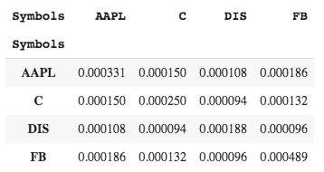
This will allow us to calculate the standard deviation and mean of returns across the entire portfolio.

3) Calculate the portfolio mean and standard deviation

# Calculate mean returns for each stock
avg_rets = returns.mean()

# Calculate mean returns for portfolio overall, 
# using dot product to 
# normalize individual means against investment weights
 # https://en.wikipedia.org/wiki/Dot_product#:~:targetText=In%20mathematics%2C%20the%20dot%20product,and%20returns%20a%20single%20number.
port_mean = avg_rets.dot(weights)

# Calculate portfolio standard deviation
port_stdev = np.sqrt(weights.T.dot(cov_matrix).dot(weights))

# Calculate mean of investment
mean_investment = (1+port_mean) * initial_investment

# Calculate standard deviation of investmnet
stdev_investment = initial_investment * port_stdev

Next, we can plug these variables into our percentage point function (PPF) below:

4) Calculate the inverse of the normal cumulative distribution (PPF) with a specified confidence interval, standard deviation, and mean

# Select our confidence interval (I'll choose 95% here)
conf_level1 = 0.05

# Using SciPy ppf method to generate values for the
# inverse cumulative distribution function to a normal distribution
# Plugging in the mean, standard deviation of our portfolio
# as calculated above
# https://docs.scipy.org/doc/scipy/reference/generated/scipy.stats.norm.html
from scipy.stats import norm
cutoff1 = norm.ppf(conf_level1, mean_investment, stdev_investment)

5) Estimate the value at risk (VaR) for the portfolio by subtracting the initial investment from the calculation in step 4

#Finally, we can calculate the VaR at our confidence interval
var_1d1 = initial_investment - cutoff1
var_1d1

#output
#22347.7792230231

Here we are saying with 95% confidence that our portfolio of 1M USD will not exceed losses greater than 22.3k USD over a one day period.

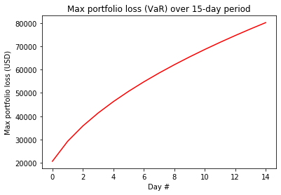
Value at risk over n-day time period

What if we wanted to calculate this over a larger window of time? Below we can easily do that by just taking our 1 day VaR and multiplying it by the square root of the time period (this is due to the fact that the standard deviation of stock returns tends to increase with the square root of time).

# Calculate n Day VaR
var_array = []
num_days = int(15)
for x in range(1, num_days+1):    
    var_array.append(np.round(var_1d1 * np.sqrt(x),2))
    print(str(x) + " day VaR @ 95% confidence: " + str(np.round(var_1d1 * np.sqrt(x),2)))

# Build plot
plt.xlabel("Day #")
plt.ylabel("Max portfolio loss (USD)")
plt.title("Max portfolio loss (VaR) over 15-day period")
plt.plot(var_array, "r")

1 day VaR @ 95% confidence: 20695.24
2 day VaR @ 95% confidence: 29267.49
3 day VaR @ 95% confidence: 35845.21
4 day VaR @ 95% confidence: 41390.49
5 day VaR @ 95% confidence: 46275.97
6 day VaR @ 95% confidence: 50692.79
7 day VaR @ 95% confidence: 54754.47
8 day VaR @ 95% confidence: 58534.99
9 day VaR @ 95% confidence: 62085.73
10 day VaR @ 95% confidence: 65444.11
11 day VaR @ 95% confidence: 68638.36
12 day VaR @ 95% confidence: 71690.43
13 day VaR @ 95% confidence: 74617.76
14 day VaR @ 95% confidence: 77434.51
15 day VaR @ 95% confidence: 80152.33

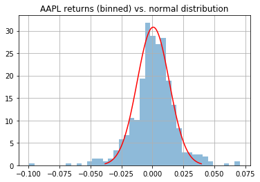
(Extra) Checking distributions of our equities against normal distribution

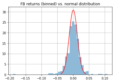
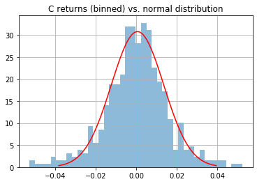
As mentioned in the calculation section, we are assuming that the returns of the equities in our portfolio are normally distributed when calculating VaR. Of course, we can't predict that moving forward, but we can at least check how the historical returns have been distributed to help us assess whether VaR is suitable to use for our portfolio.

import matplotlib.mlab as mlab
import matplotlib.pyplot as plt
# Repeat for each equity in portfolio
returns['AAPL'].hist(bins=40, normed=True,histtype="stepfilled",alpha=0.5)
x = np.linspace(port_mean - 3*port_stdev, port_mean+3*port_stdev,100)
plt.plot(x, scipy.stats.norm.pdf(x, port_mean, port_stdev), "r")
plt.title("AAPL returns (binned) vs. normal distribution")
plt.show()

AAPl returns vs. normal distribution

FB returns vs. normal distribution

C returns vs. normal distribution

DIS returns vs. normal distribution

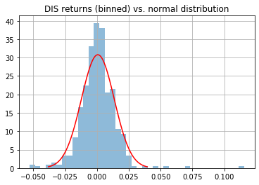
From the above we can see the returns have all been fairly normally distributed for our chosen stocks since 2018.

//You can view the code in Google Colab here - to run it just make a copy of the notebook.