St. Petersburg Paradox

The St. Petersburg Paradox is a paradox related to probability and decision theory in economics. It is based on a lottery game that has an infinite expected value (one should be willing to play at whatever cost). However, for the participants, each game is only worth a small amount (hence the paradox). This post will go over the expected value of a game, the reality of the expected value, and a Python simulation to emphasize the game's reality.

The standard version of the St. Petersburg Paradox is derived from the St. Petersburg game. The game is played by flipping a fair coin until a heads appears (at which point the game is over). The player wins $2 per flip. Given the rules of the game, what would be a fair price to enter the game?

Solving for cost using expected value

We can use probability theory to solve for the expected value of the game, then assume any price less than the expected value is a fair price. The expected value of the game is straightforward to calculate. All that is needed is the monetary values of the outcomes and their probabilities. If the coin lands heads on the first flip, winnings are $2. If it lands heads on the second flip, winnings are $4. If this happens on the third flip, winnings are $8, and so on.

The probabilities of the outcomes are (\frac{1}{2}\ ), (\frac{1}{4}\ ), (\frac{1}{8}\ ), etc.

Given this, the expected monetary value of the St. Petersburg game is:

(E(X) = (\frac{1}{2}\ \times2) + (\frac{1}{4}\ \times4) + (\frac{1}{8}\ \times8) + (\frac{1}{16}\ \times16) + \ldots )

( E(X) = \sum_{n=1}^{\infty} (\frac{1}{2})^{n} \cdot 2^n )

(E(X) = \infty )

The probabilistic expected value of the game is infinite, meaning any cost would be acceptable to play the game. For many reasons this does not make sense, and we'll go into the reality of the game in the next section.

Reality of the expected value

The expected value of the game indicates that it would be rational to pay any amount for an opportunity to play the game, even though average payout of the game is quite low. For example, there's a 50% chance of winning $2, and a 75% chance that no more than $4 will be won. Given the two statistics and potential winnings, the reality is that individuals are probably not willing to pay more than $2-4 dollars to play this game. We can support this hypothesis in the next section with a simulation.

Simulating the game

Here is a link to the simulation of the game in a Python notebook. You can create a copy of this notebook and run the simulation yourself. In the simulation, 100,000 iterations of the game were run and yielded the following outputs:

Total Winnings: 751340 Expected Winnings: 7.5134 Median Winnings: 2.0

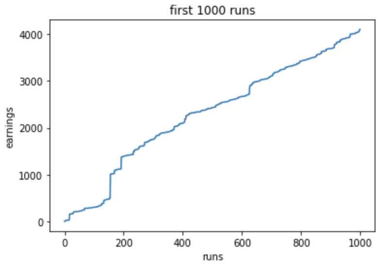
The output of the simulation provides a framework to come up with a more reasonable cost per game. From the simulation, the expected winnings per game is $7.51, however the median expected winnings are $2.00 per game. As we stated above, we have a 50% chance of winning $2, and the median winnings of $2 from our simulation make sense. The expected winnings are much higher than the median, but again this is after playing the game 100,000 times (which a person probably will not be playing the game for that long). The chart below plots the first 1000 runs and the cumulative winnings. At 200 runs, our simulation has us at ~$800 of winnings, and at 1000 runs, our simulation has us at $5000. This places the value of our game between $4-$5 per game. We would want to err on the conservative side of $4 per game, and we can estimate that one would only want to pay less than $4 per game.

Below is the code that is used in the notebook and an example of the output for 100,000 runs:

#importing packages
import numpy as np
from scipy import stats

def GameTime(n_simulations):
  win = 0
  win_list = []
  for i in range(n_simulations):
      coin = 1
      n_consecutive_heads = 0

      while coin == 1:
          #creating binomial distribution for flip
          coin = np.random.binomial(1, 0.5)
          #if coin toss is = 1, then we keep going and
          # count the # of consecutive tails
          if coin == 1:
              n_consecutive_heads += 1

      #we enter this when we break our streak
      # if we get more than 1 head...
      if n_consecutive_heads != 0:
          #...we calculate our winnings
          new_win = 2 ** n_consecutive_heads
          #and append it to our running total for the simulation
          win += new_win
          #and append the instance to a list
          win_list.append(new_win)
      else:
          #if we lose, we append $0
          win_list.append(0)

  win_list = np.array(win_list, dtype=np.int32)
  print("Total Winnings:", win)
  print("Expected Winnings:", win / n_simulations)
  print("Median Winnings:", np.median(win_list), "\n")

  bins = np.bincount(win_list)
  unique = np.unique(win_list)

  for u in unique:
      print("Won ${}: {} times".format(u, bins[u]))

#driver code
n_simulations = 100000
GameTime(n_simulations)

Output:

Total Winnings: 751340
Expected Winnings: 7.5134
Median Winnings: 2.0

Won $0: 49769 times
Won $2: 25216 times
Won $4: 12515 times
Won $8: 6334 times
Won $16: 3075 times
Won $32: 1586 times
Won $64: 756 times
Won $128: 370 times
Won $256: 200 times
Won $512: 94 times
Won $1024: 52 times
Won $2048: 13 times
Won $4096: 9 times
Won $8192: 7 times
Won $16384: 2 times
Won $32768: 1 times
Won $65536: 1 times