Bayesian Analysis of The Price is Right Showcase

August 2020

1) The rules of The Price is Right / the setup

Suppose we're a contestant on a popular game show called The Price is Right. We've made it to 'The Showcase' round where we're tasked with guessing the price of a group of prizes (typically trips, cars, furniture, etc.). The rules for the round (simplified a bit for our example) are as follows:

There are two contestants competing in a showcase round
Both contestants are shown unique groups of prizes (two groups of prizes shown in total)
After seeing the prizes, each contestant is asked to bid on what they think the value is of their unique set of prizes
Whichever bid is closer, without going over, wins. If a contestant bids over, then their bid is disqualified from winning

This game provides an interesting example of balancing uncertainty with risk (since if we bid even 1 dollar over the true price of the items we are disqualified).

Given this information, we'll step through using Bayesian Inference to build a model and select our final bid in the showcase. Below are some details for our hypothetical showcase round (the exact #s are not important):

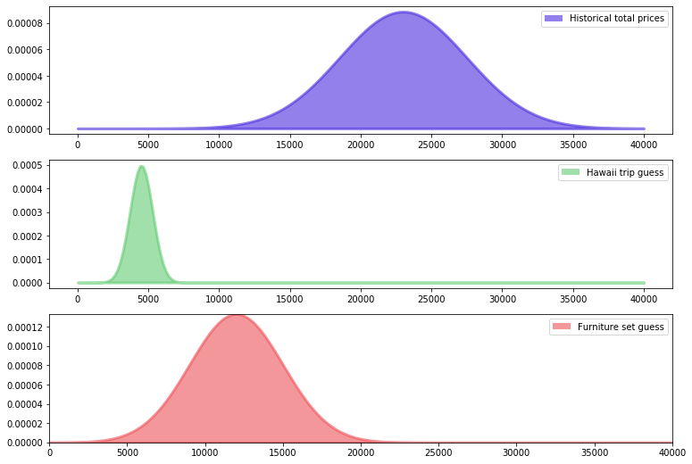
We'll assume we have data on the 'true prices' of past The Price is Right Showcase prizes, and they are normally distributed with a mean of 23,000 and a standard deviation of 4,500
The two prizes in our prize package are:
- A trip to Hawaii
- A set of living room furniture

2) Visualizing the historical 'true price' distribution, along with our guesses

First, we'll set up a quick visualization to illustrate the historical 'true price,' as well as our guesses for each sub-prize in our package:

# Import libraries
%matplotlib inline
import scipy.stats as stats
from IPython.core.pylabtools import figsize
import numpy as np
import matplotlib.pyplot as plt

figsize(12.5, 9)

### Plot historical total price distribution ###

##################################################
# Subplot 1: historical total package true prices
# 3 x 1 grid, first sub plot
plt.subplot(311)
# Set range for x-axis
# 0-40000, split into 200 intervals
x = np.linspace(0, 40000, 200)
# Set up plot, normally distributed pdf 
# with mean of 23000, std. dev of 4500
# set up line color, weight, alpha (opacity), 
# line label
sp1 = plt.fill_between(x , 0, stats.norm.pdf(x, 23000, 4500), 
                color = "#4b2cde", lw = 3, alpha = 0.6,
                label = "Historical total prices")
# Plot subplot inside rectangle, starting at 0,0 width/height of 1
p1 = plt.Rectangle((0, 0), 1, 1, fc=sp1.get_facecolor()[0])
# Add legend
plt.legend([p1], [sp1.get_label()])

##################################################

# Subplot 2: Our guess for Hawaii trip cost
# Comments repeat for historical price distribution above
plt.subplot(312)
x = np.linspace(0, 40000, 200)
sp2 = plt.fill_between(x , 0, stats.norm.pdf(x, 4500, 800), 
                 color = "#62cb73", lw = 3, alpha = 0.6,
                 label="Hawaii trip guess")

p2 = plt.Rectangle((0, 0), 1, 1, fc=sp2.get_facecolor()[0])
plt.legend([p2], [sp2.get_label()])

##################################################

# Subplot 3: Our guess for living room furniture
plt.subplot(313)
x = np.linspace(0, 40000, 200)
sp3 = plt.fill_between(x , 0, stats.norm.pdf(x, 12000, 3000), 
                 color = "#ed5259", lw = 3, alpha = 0.6,
                 label = "Furniture set guess")
plt.autoscale(tight=True)
p3 = plt.Rectangle((0, 0), 1, 1, fc=sp3.get_facecolor()[0])
plt.legend([p3], [sp3.get_label()]);

3) Plug our guesses + historical price information into a Bayesian statistical model

Next, we'll feed our guesses, as well as the historical total price mean and standard deviation, into PyMC3 (a Python package for Bayesian statistical modeling and probabilistic machine learning).

# Import library
import pymc3 as pm
# Mean guesses: Hawaii trip, furniture
data_mu = [4500, 12000]
# Our error estimate on guesses: Hawaii trip, furniture
data_std =  [800, 3000] 
# Historical mean
mu_prior = 23000
# Historical standard deviation
std_prior =  4500

# If new to pymc3, would recommend exploring quickstart/docs:
# https://docs.pymc.io/notebooks/api_quickstart.html
with pm.Model() as model:
    # Feed the variables into our model
    # you can read more about the required variables/structure
    # in the docs above
    true_price = pm.Normal("true_price", mu=mu_prior, sd=std_prior)
    prize_1 = pm.Normal("first_prize", mu=data_mu[0], sd=data_std[0])
    prize_2 = pm.Normal("second_prize", mu=data_mu[1], sd=data_std[1])
    price_estimate = prize_1 + prize_2
    # Here we're evaluating a normal distribution w/ mean of price_estimate,
    # standard deviation of 3800, at the values provided by true_price
    # PyMC3 expects the logp() method to return a log-probability 
    # evaluated at the passed value argument. This method is used 
    # internally by all of the inference methods to calculate the model 
    # log-probability that is used for fitting models. 
    logp = pm.Normal.dist(mu=price_estimate, sd=(3800)).logp(true_price)
    error = pm.Potential("error", logp)

    # Set step method, pull sample
    # Here we selected NUTS, 'No-U-Turn Sampler' most commonly used
    # in pymc3, Markov chain Monte Carlo sampling algorithm
    trace = pm.sample(50000, step=pm.NUTS())
    # Sampler usually converge to the typical set slowly in high dimension, 
    # generally good practice to discard first few thousand samples that are 
    # not yet in the typical set. Less of an issue with modern sampler like NUTS
    burned_trace = trace[10000:]

true_price_trace = burned_trace["true_price"]

4) Plot our new price estimate along with the prior distribution of historical prices

Next we can plot the output of our 'price_trace' which represents our new price estimate. Additionally, we'll plot the distribution and mean of the prior (historical) estimate so we can visually see how things shifted:

import scipy.stats as stats
# Build linespace from 5000-40000 for 
# x axis
x = np.linspace(5000, 40000)
# Plot normal pdf for historical prior distribution
plt.plot(x, stats.norm.pdf(x, 23000, 4500), c = "k", lw = 2, 
         label = "prior dist. of suite price")
# Plot price trace into histogram, add lines for mean, prior's mean
_hist = plt.hist(true_price_trace, bins = 25, normed= True, color = "#4b2cde", alpha=0.6, histtype= "stepfilled")
plt.title("Posterior of the true price estimate")
plt.vlines(mu_prior, 0, 1.1*np.max(_hist[0]), label = "prior's mean",
           linestyles="--")
plt.vlines(true_price_trace.mean(), 0, 1.1*np.max(_hist[0]), \
           label = "posterior's mean", linestyles="-.")
plt.legend(loc = "upper right");

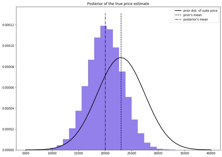
Here we can see that due to our two observed prizes and guesses (including our uncertainty estimates expressed as standard deviation), we shifted our mean price estimate down a few thousand dollars from the prior mean price.

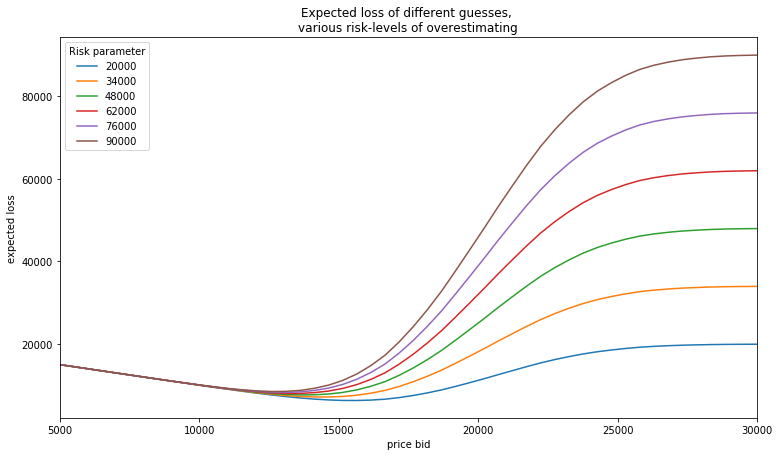
5) Account for the asymmetric reward system for our guesses

Now that we've adjusted our bid from just pulling the mean of prior distributions (23,000), one might be tempted to just take our new posterior mean that incorporates our estimates for each prize into the overall bid.

However, we can incorporate one more factor - risk - into our thinking before arriving at a final bid.

Since the rules of the game are unique in the sense that any bid over the value results in earnings of $0, we can create a loss function to incorporate a 'risk' parameter, which is meant to represent how bad it is for us if we guess higher than the true price. (A proxy for our risk aversion)

For every possible bid, we calculate the expected loss associated with that bid. We then vary the risk parameter to see how it affects our loss:

figsize(12.5, 7)
#numpy friendly showdown_loss

def showdown_loss(guess, true_price, risk = 80000):
        loss = np.zeros_like(true_price)
        ix = true_price < guess
        loss[~ix] = np.abs(guess - true_price[~ix])
        loss[ix] = risk
        return loss

# x-axis labeling
guesses = np.linspace(5000, 40000, 70) 
# y-axis labeling, risk band
risks = np.linspace(20000, 90000, 6)
expected_loss = lambda guess, risk: \
    showdown_loss(guess, true_price_trace, risk).mean()

# Loop through each risk parameter, calculate the expected 
# loss, plot        
for _p in risks:
    results = [expected_loss(_g, _p) for _g in guesses]
    plt.plot(guesses, results, label = "%d"%_p)

plt.title("Expected loss of different guesses, \nvarious risk-levels of \
overestimating")
plt.legend(loc="upper left", title="Risk parameter")
plt.xlabel("price bid")
plt.ylabel("expected loss")
plt.xlim(5000, 30000);

6) Minimize our expected loss, calculate our bid across various risk levels

Here we can visually see approximations for where the minimum expected loss is relative to each risk parameter (line). However, we can get more precise by plugging this into an optimization function and minimizing our expected loss subject to our risk.

The function in 'fmin in scipy.optimize' module uses an intelligent search to find a minimum (not necessarily a global minimum) of any uni or multivariate function. For most purposes, 'fmin' will provide you with a good answer. Note there are several ways to pull the rough minimum out of this function, this is just a quick approach:

import scipy.optimize as sop
ax = plt.subplot(111)
for _p in risks:
    _color = next(ax._get_lines.prop_cycler)
    # https://docs.scipy.org/doc/scipy/reference/generated/scipy.optimize.fmin.html
    # 10k is our x0, starting point
    _min_results = sop.fmin(expected_loss, 10000, args=(_p,),disp = False)
    _results = [expected_loss(_g, _p) for _g in guesses]
    plt.plot(guesses, _results , color = _color['color'])
    plt.scatter(_min_results, 0, s = 60, \
                color= _color['color'], label = "%d"%_p)
    plt.vlines(_min_results, 0, 120000, color = _color['color'], linestyles="--")
    print("minimum at risk %d: %.2f" % (_p, _min_results))

plt.title("Expected loss & Bayes actions of different guesses, \n \
various risk-levels of overestimating")
plt.legend(loc="upper left", scatterpoints = 1, title = "Bayes action at risk:")
plt.xlabel("price guess")
plt.ylabel("expected loss")
plt.xlim(6000, 30000)
plt.ylim(0, 100000);

minimum at risk 20000: 15507.21
minimum at risk 34000: 14336.10
minimum at risk 48000: 13817.60
minimum at risk 62000: 13353.86
minimum at risk 76000: 12932.99
minimum at risk 90000: 12930.03

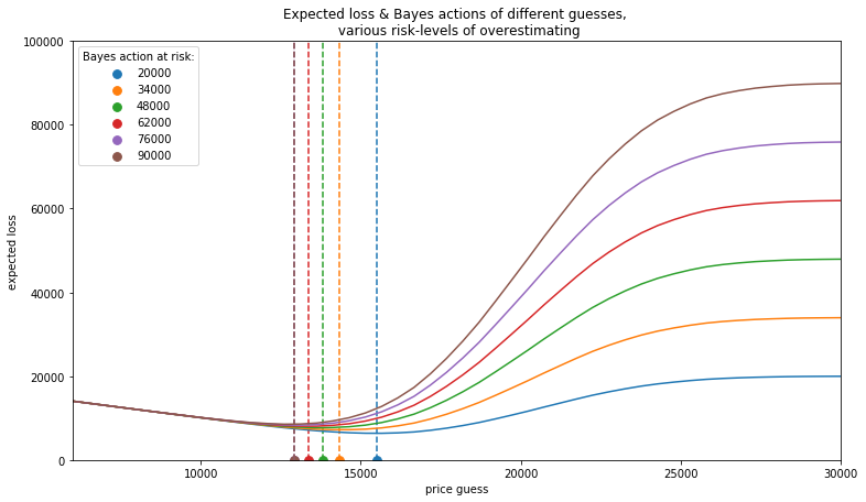
As expected, when we decrease the risk threshold, our optimal bid increases. Additionally, we can see that the overall bid is shifted lower (compared to the posterier mean above) when accounting for risk, which is in line with a realistic strategy one would undertake in this game. In other words, we'd expect someone with a level of risk aversion to slightly undercut their normal price estimate to avoid overbidding. So depending on our personal risk level, we can now select our best estimate for the showcase!