Introduction to Linear Regression using Python

December 2019

This post will walk through a practice problem which analyzes NBA players' season stats. We've also provided the practice problem's Colab Notebook so you can follow along. Just copy the notebook and the two Google sheets (season stats and player data) to your Google Drive.

This practice problem has a data set that contains NBA players and their invidiual season stats. This practice will take you through fitting a linear model using player stats to estimate win shares per 48 minutes.

Topics covered in this tutorial:

Importing data from Google Sheets into Colab
Basic data cleaning / analysis
Splitting data into test and training sets
Training a single variable regression model
Training a multivariate regression model
Manually calculating Adjusted R-squared and R-squared
Calculating Root Mean Square Error
Comparing results of 2 regression models

Importing and cleaning data

# Importing packages.
import pandas as pd
import matplotlib.pyplot as plt
import seaborn as sb
import numpy as np
import scipy.stats as ss
from sklearn.linear_model import LinearRegression
import seaborn as sns
sns.set(color_codes = True)
%matplotlib inline

# Setting figure sizes
plt.rcParams['figure.figsize'] = (8, 6)
plt.rcParams['font.size'] = 14

# Code to connect Colab to Google Drive (save the spreadsheet provided into your drive)
# https://colab.research.google.com/notebooks/io.ipynb#scrollTo=JiJVCmu3dhFa

!pip install --upgrade -q gspread
from google.colab import auth
auth.authenticate_user()

import gspread
from oauth2client.client import GoogleCredentials

gc = gspread.authorize(GoogleCredentials.get_application_default())

### Importing sheet

# Open our new sheet and read some data.
worksheet = gc.open('Seasons_Stats').sheet1
# get_all_values gives a list of rows.
rows = worksheet.get_all_values()
# Convert to a DataFrame and render.
seasonPlayerStats = pd.DataFrame.from_records(rows)

### Fixing header of dataframe

# our header isn't named correctly lets fix our header
seasonPlayerStats.columns = seasonPlayerStats.iloc[0]
#drop the first row after we rename the header
seasonPlayerStats = seasonPlayerStats.reindex(seasonPlayerStats.index.drop(0))

### Importing sheet

# Open our new sheet and read some data.
worksheet = gc.open('player_data').sheet1
# get_all_values gives a list of rows.
rows = worksheet.get_all_values()
# Convert to a DataFrame and render.
playerData = pd.DataFrame.from_records(rows)

### Fixing header of dataframe
#rename header so it's the first row
playerData.columns = playerData.iloc[0]
#drop the first row after we rename the header
playerData = playerData.reindex(playerData.index.drop(0))

# Merging dataframes and dropping null values so we avoid errors
# joining 
playerAllStats = pd.merge(seasonPlayerStats, playerData, how='left', on='Player')
# dropping null value columns to avoid errors 
playerAllStats = playerAllStats[pd.notnull(playerAllStats['height'])]
playerAllStats = playerAllStats[pd.notnull(playerAllStats['Points'])]
playerAllStats = playerAllStats[pd.notnull(playerAllStats['Games'])]
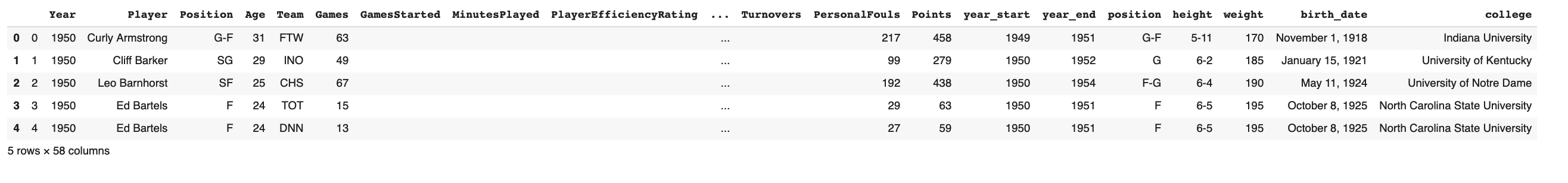
playerAllStats.head()

Output:

#Viewing all columns that we have in the dataframe. I'll be referencing this figure out which fields I need to clean
playerAllStats.columns

Output:


Index(['', 'Year', 'Player', 'Position', 'Age', 'Team', 'Games',
   'GamesStarted', 'MinutesPlayed', 'PlayerEfficiencyRating',
   'TrueShootingPerct', 'ThreePointAttemptRate', 'FreeThrowRate',
   'OffensiveReboundPercentage', 'DefensiveReboundPercentage',
   'TotalReboundPercentage', 'AssistPercentage', 'StealPercentage',
   'BlockPercentage', 'TurnoverPercentage', 'UsagePercentage',
   'OffesniveWinShares', 'DefensiveWinShares', 'WinShares',
   'WinsSharesPer48Minutes', 'OffensiveBoxPlusMinus',
   'DefensiveBoxPlusMinus', 'BoxPlusMinus', 'ValueOverReplacement',
   'FieldGoals', 'FieldGoalAttempts', 'FieldGoalPercentage',
   'ThreePointFieldGoals', 'ThreePointFieldGoalAttempts',
   'ThreePointFieldGoalPercentage', 'TwoPointFieldGoals',
   'TwoPointFieldGoalAttempts', 'TwoPointFieldGoalPercentage',
   'EffectiveFieldGoalPercentage', 'FreeThrows', 'FreeThrowAttempts',
   'FreeThrowPercentage', 'OffensiveRebounds', 'DefensiveRebounds',
   'TotalRebounds', 'Assists', 'Steals', 'Blocks', 'Turnovers',
   'PersonalFouls', 'Points', 'year_start', 'year_end', 'position',
   'height', 'weight', 'birth_date', 'college', 'feet', 'inches',
   'heightInches', 'PointsPerGame', 'TotalReboundsPerGame',
   'AssistsPerGame'],
  dtype='object', name=0)

Cleaning data even more

Converting height to inches (so we can use it if we decide to)
Converting some of the stats to a numeric value so we can do analysis
Calculating points per game, total rebounds per game, and assists per game

playerAllStats['feet'], playerAllStats['inches'] = playerAllStats['height'].str.split('-', 1).str
playerAllStats['feet'], playerAllStats['inches'], playerAllStats['weight'] = pd.to_numeric(playerAllStats.feet), \
  pd.to_numeric(playerAllStats.inches), pd.to_numeric(playerAllStats.weight)
playerAllStats['heightInches'] = playerAllStats['feet']*12 + playerAllStats['inches']

playerAllStats['Games'], playerAllStats['Points'] = pd.to_numeric(playerAllStats.Games), pd.to_numeric(playerAllStats.Points)
playerAllStats['MinutesPlayed'], playerAllStats['FieldGoalPercentage']= pd.to_numeric(playerAllStats.MinutesPlayed), pd.to_numeric(playerAllStats.FieldGoalPercentage)
playerAllStats['Games'], playerAllStats['TotalRebounds']= pd.to_numeric(playerAllStats.Games), pd.to_numeric(playerAllStats.TotalRebounds)
playerAllStats['Assists'], playerAllStats['WinsSharesPer48Minutes']= pd.to_numeric(playerAllStats.Assists), pd.to_numeric(playerAllStats.WinsSharesPer48Minutes)
playerAllStats['WinShares'], playerAllStats['Year'] = pd.to_numeric(playerAllStats.WinShares), pd.to_numeric(playerAllStats.Year)

playerAllStats['PointsPerGame'] = playerAllStats['Points']/ playerAllStats['Games']
playerAllStats['TotalReboundsPerGame'] = playerAllStats['TotalRebounds']/ playerAllStats['Games']
playerAllStats['AssistsPerGame'] = playerAllStats['Assists']/ playerAllStats['Games']

Question: Can we create a linear regression model using points per game to estimate win shares per 48 minutes? 1. Create a plot with the 2 statistics Before we create the model, let's plot the points per game vs win shares per 48 minutes. This will let us understand the data set and see if we need to remove outliers to improve model accuracy.

sns.regplot(x="WinsSharesPer48Minutes", y = "PointsPerGame", data=playerAllStats)

Output:

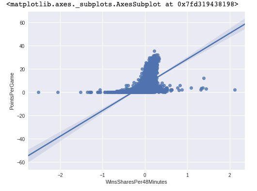
There's obviously some outliers and data that doesn't belong. Let's see what kind of data we're working with.

playerAllStats.describe()

Output: 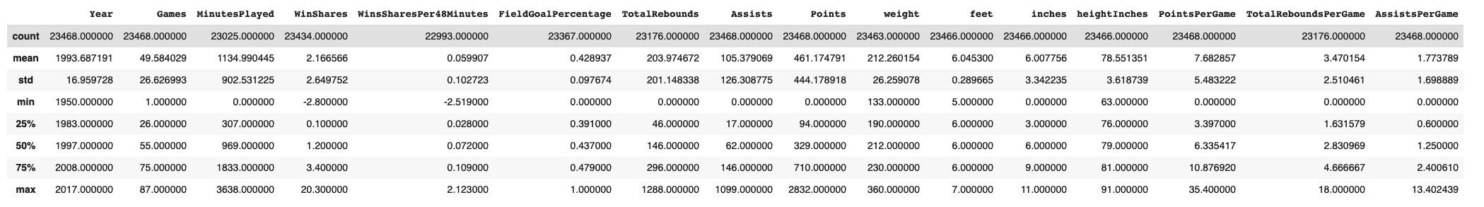There's a few things I see immediately that would make our data hard to plot.

We have seasons from 11400...to minimize noise, we're only going to look at recent player's seasons. So I'm going to limit my analysis from 2014 to present.
We have players who've played 1 game all season. We're also going to limit the number of games a player has played in a given season to be >70% of all games. A given season has 82 games.
This isn't in the descriptive statistics above, but there are different positions in basketball. For the purpose of this analysis let's limit our data to include players who play Point Guard (PG) (or other positions along with PG). These are typically the players who score the most points, and it makes sense for us to group players who have even scoring potential to reduce skewness.

#filtering on players who have played since 2014 and have played at least 70% of the games in a given season (assuming 82 games per season)
playerAllStatsSince2014 = playerAllStats.loc[(playerAllStats['Year'] >= 2014) &(playerAllStats['Games'] >= 58)] 
#filteirng on PG players
playerAllStatsSince2014PG = playerAllStatsSince2014[playerAllStatsSince2014['Position'].str.contains('PG')].reset_index(drop=True)
sns.regplot(x="WinsSharesPer48Minutes", y = "PointsPerGame", data=playerAllStatsSince2014PG)

Output: 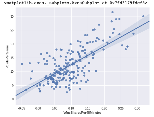The plot looks much better between points per game vs win shares per 48 minutes. Our data is in a format we can use. Let's move on to creating a training and test data set.

2. Splitting data into training and test set We're going to split our data into dependent variables and an independent varaibles for both training and test sets using SKLearn's 'train_test_split' function.

playerAllStatsSince2014PG_WinShare = playerAllStatsSince2014PG['WinsSharesPer48Minutes']
playerAllStatsSince2014PG_PPG = playerAllStatsSince2014PG['PointsPerGame']

 #importing packages and splitting out data into training + testing sets
from sklearn.model_selection import train_test_split
train_x, test_x, train_y, test_y = train_test_split(playerAllStatsSince2014PG['PointsPerGame'], \
                                              playerAllStatsSince2014PG['WinsSharesPer48Minutes'], test_size=0.20, random_state=42)

3. Fitting the data to a linear regression and getting R-squared Here we're creating a linear regression model called 'model_1.' We're going to fit the training data to this model. After that we're going to get the R-squared value. R-squared is a value between 0 and 1 which is a statistical measure of how close the data are to the fitted regression line. 1 = perfect fit, 0 = no fit

model_1 = LinearRegression()
model_1.fit(train_x.reshape(-1, 1), train_y.reshape(-1, 1))
model_1.score(train_x.reshape(-1, 1), train_y.reshape(-1, 1))

Output:

0.49632072484943907

An r-squared of 0.496 tells us we have a moderately effective fit. Since we're also going to be creating a multi-variate model, let's also calculate Adjusted R-squared and Root Mean Square Error (RMSE) so we have more statistics to compare. The below code calculates R-squared and Adjusted R-squared.

X = train_x.values.reshape(-1, 1)
y = train_y.values.reshape(-1, 1)

# compute with formulas from the theory
yhat = model_1.predict(X)
SS_Residual = sum((y-yhat)**2)
SS_Total = sum((y-np.mean(y))**2)
r_squared = 1 - np.divide(SS_Residual,SS_Total)
#r_squared = 1 - np.exp((float(SS_Residual))/SS_Total)
adjusted_r_squared = 1 - (1-r_squared)*(len(y)-1)/(len(y)-X.shape[1]-1)
print(r_squared, adjusted_r_squared)

Output:

[0.49632072] [0.49326812]

4. Estimate values for the test data Last thing to do is to estimate Win Shares with our test data. We'll compare our estimate to the true values and calculate the Root Mean Square Error.

model_1_predict_values = model_1.predict(test_x.values.reshape(-1, 1))
model_1_predict = pd.DataFrame({'Points Per Game': test_x.values, 'Actual Win Share': test_y.values,'Predicted Win Share': model_1_predict_values.reshape(1, -1)[0]})

The code below calculate Root Mean Square Error. The lower the Root Mean Square Error the closer our estimations are to the real values.

#Root Mean square error on test dataset
np.sqrt(np.mean(np.square(model_1_predict['Actual Win Share'] - \
                         model_1_predict['Predicted Win Share'])))

Output:

0.0523034857831081

Question: Can we create a linear regression model using points per game, total rebounds per game, and assists per game to estimate win shares per 48 minutes? We'll go through the same process as above (less the data exploration, which we do not need to do 2 times). We'll create the model and generate the statistics. Then we'll compare the single variable to the multivariable model.

playerAllStatsSince2014PG_Ys = playerAllStatsSince2014PG['WinsSharesPer48Minutes']
playerAllStatsSince2014PG_Xs = playerAllStatsSince2014PG[['PointsPerGame', 'TotalReboundsPerGame', 'AssistsPerGame']]

#splitting test and training data
train_x, test_x, train_y, test_y = train_test_split(playerAllStatsSince2014PG_Xs, playerAllStatsSince2014PG_Ys, test_size=0.20, random_state=42)

#fitting model
model_1 = LinearRegression()
model_1.fit(train_x, train_y)
model_1.score(train_x, train_y)

Output:

0.5060498809063979

It looks like this model's R-square value is already higher that our single variable. Next we'll calculate the model's estimate for Win Shares.

model_1_predict_values = model_1.predict(test_x)
model_1_predict = pd.DataFrame({'Actual Win Share': test_y.values,'Predicted Win Share': model_1_predict_values.reshape(1, -1)[0]})
#Root Mean square error on test dataset
np.sqrt(np.mean(np.square(model_1_predict['Actual Win Share'] - model_1_predict['Predicted Win Share'])))

Output:

0.05174714479057624

X = train_x.values
y = train_y.values

# compute with formulas from the theory
yhat = model_1.predict(X)
SS_Residual = sum((y-yhat)**2)
SS_Total = sum((y-np.mean(y))**2)
r_squared = 1 - np.divide(SS_Residual,SS_Total)
#r_squared = 1 - np.exp((float(SS_Residual))/SS_Total)
adjusted_r_squared = 1 - (1-r_squared)*(len(y)-1)/(len(y)-X.shape[1]-1)
print(r_squared, adjusted_r_squared)

Output:

0.5060498809063977 0.49695877442001235

Comparing single variable to multivariate linear regression model Below is a summary of the test statistics of the two models we created. Across all 3 statistics, the multivariate model performs slightly better than the single variable.

statistic	single	multi
r-squared	0.49632	0.50604
adjusted r-squared	0.49326	0.49695
RMSE	0.0523	0.0517