Simulating Future Stock Prices using Monte Carlo Methods in Python

Using Monte Carlo methods, we'll write a quick simulation to predict future stock price outcomes for Apple ($AAPL) using Python. You can read more about Monte Carlo simulation (in a finance context) here.

1) Pull the data

First, we can import the libraries, and pull the historical stock data for Apple. For this example, I picked the last ~10 years, although it would be valuable to test sensitivities of different ranges as this alone is subjective:

# Import required libraries
import math
import matplotlib.pyplot as plt
import numpy as np
from pandas_datareader import data
apple = data.DataReader('AAPL', 'yahoo',start='1/1/2009')
apple.head()

	High	Low	Open	Close	Volume	Adj Close
Date
2009-01-02	13.005714	12.165714	12.268572	12.964286	186503800.0	11.357091
2009-01-05	13.740000	13.244286	13.310000	13.511429	295402100.0	11.836406
2009-01-06	13.881429	13.198571	13.707143	13.288571	322327600.0	11.641174
2009-01-07	13.214286	12.894286	13.115714	13.001429	188262200.0	11.389630
2009-01-08	13.307143	12.862857	12.918571	13.242857	168375200.0	11.601127

#Next, we calculate the number of days that have elapsed in our chosen time window
time_elapsed = (apple.index[-1] - apple.index[0]).days

2) Calculate the compounded annualized growth rate over the length of the dataset + standard deviation (to feed into simulation)

#Current price / first record (e.g. price at beginning of 2009)
#provides us with the total growth %
total_growth = (apple['Adj Close'][-1] / apple['Adj Close'][1])

#Next, we want to annualize this percentage
#First, we convert our time elapsed to the # of years elapsed
number_of_years = time_elapsed / 365.0
#Second, we can raise the total growth to the inverse of the # of years
#(e.g. ~1/10 at time of writing) to annualize our growth rate
cagr = total_growth ** (1/number_of_years) - 1

#Now that we have the mean annual growth rate above,
#we'll also need to calculate the standard deviation of the
#daily price changes
std_dev = apple['Adj Close'].pct_change().std()

#Next, because there are roughy ~252 trading days in a year,
#we'll need to scale this by an annualization factor
#reference: https://www.fool.com/knowledge-center/how-to-calculate-annualized-volatility.aspx

number_of_trading_days = 252
std_dev = std_dev * math.sqrt(number_of_trading_days)

#From here, we have our two inputs needed to generate random
#values in our simulation
print ("cagr (mean returns) : ", str(round(cagr,4)))
print ("std_dev (standard deviation of return : )", str(round(std_dev,4)))

cagr (mean returns) : 0.3746 std_dev (standard deviation of return : ) 0.2878

3) Generate random values, run Monte Carlo simulation

#Generate random values for 1 year's worth of trading (252 days),
#using numpy and assuming a normal distribution
daily_return_percentages = np.random.normal(cagr/number_of_trading_days, std_dev/math.sqrt(number_of_trading_days)number_of_trading_days)+1

#Now that we have created a random series of future
#daily return %s, we can simply apply these forward-looking
#to our last stock price in the window, effectively carrying forward
#a price prediction for the next year

#This distribution is known as a 'random walk'

price_series = [apple['Adj Close'][-1]]

for j in daily_return_percentages:
    price_series.append(price_series[-1] * j)

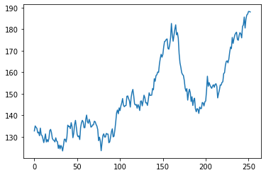
#Great, now we can plot of single 'random walk' of stock prices
plt.plot(price_series)
plt.show()

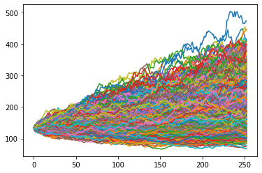
#Now that we've created a single random walk above,
#we can simulate this process over a large sample size to
#get a better sense of the true expected distribution
number_of_trials = 3000

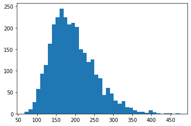
#set up an additional array to collect all possible
#closing prices in last day of window.
#We can toss this into a histogram
#to get a clearer sense of possible outcomes
closing_prices = []

for i in range(number_of_trials):
    #calculate randomized return percentages following our normal distribution
    #and using the mean / std dev we calculated above
    daily_return_percentages = np.random.normal(cagr/number_of_trading_days, std_dev/math.sqrt(number_of_trading_days),number_of_trading_days)+1
    price_series = [apple['Adj Close'][-1]]

    for j in daily_return_percentages:
        #extrapolate price out for next year
        price_series.append(price_series[-1] * j)

    #append closing prices in last day of window for histogram
    closing_prices.append(price_series[-1])

    #plot all random walks
    plt.plot(price_series)

plt.show()

#plot histogram
plt.hist(closing_prices,bins=40)

plt.show()

4) Analyze results

#from here, we can check the mean of all ending prices
#allowing us to arrive at the most probable ending point
mean_end_price = round(np.mean(closing_prices),2)
print("Expected price: ", str(mean_end_price))

Expected price: 193.85

#lastly, we can split the distribution into percentiles
#to help us gauge risk vs. reward

#Pull top 10% of possible outcomes
top_ten = np.percentile(closing_prices,100-10)

#Pull bottom 10% of possible outcomes
bottom_ten = np.percentile(closing_prices,10);

#create histogram again
plt.hist(closing_prices,bins=40)
#append w/ top 10% line
plt.axvline(top_ten,color='r',linestyle='dashed',linewidth=2)
#append w/ bottom 10% line
plt.axvline(bottom_ten,color='r',linestyle='dashed',linewidth=2)
#append with current price
plt.axvline(apple['Adj Close'][-1],color='g', linestyle='dashed',linewidth=2)

plt.show()

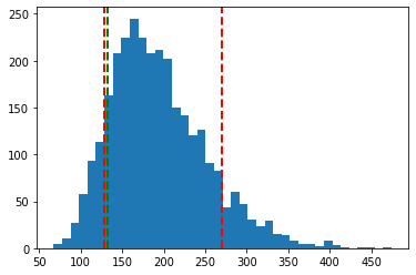
Here, we can see (based solely on using Monte Carlo simulation, of course) there looks to be more upside than downside for the next year, with the expected price running about $193 and only a 10% chance of the price landing below $128.

There are of course many, many things that drive a stock price beyond historical percent changes (meaning I would not make investment decisions solely off Monte Carlo simulation!), but this offers a thorough example of using Monto Carlo simulation to better understand the distribution of possible outcomes.